#Learning around mistakes
Jev has taken over the twitterverse with its speed and efficiency, and I’ve seen some great demos on Twitter lately. A couple nights ago, I was scrolling Twitter like I often do, and I saw a demo by Mustafa where he used Jev to make a NAND gate. He then wired enough of them together to run a 4-bit ALU.
Jev is TypeSafe AI’s frozen evaluation model, so every gate was an API call. By his numbers, 7 + 5 = 12 took 116 gates, 7.6 seconds and $0.0018, with an 84% compound probability that the answer came out right.
He built it as a joke to say that billions of these will eventually power Doom one day, but this demo got me thinking of any way I can do something even sillier. Mustafa’s ALU got me thinking about the classic first neural net, the one that learns to read handwritten digits. What if every neuron in it was a Jev call?
His ALU had fixed wiring, so when a gate misfired, the answer was wrong and nothing in the circuit could correct it. A neural network’s wiring is learned, and I wanted to know whether the weights around an imperfect neuron could learn to compensate for its mistakes.
To find out, I built Jevrons, a small neural network where every neuron is a live Jev call, and trained it with backprop to read handwritten digits. I started with a single neuron and built up to a full digit classifier, and most of the experiments along the way came out of something the previous one turned up.
The TLDR of this silly experiment is that when every neuron (Jev call) has to add a long list, a network trained with perfect arithmetic falls apart on Jev, dropping from 84% to 53% accuracy on ten digits. The coolest part is that the weights learned to work around Jev’s arithmetic mistakes!
#Defining a Jevron
Some background for the uninitiated:
Jev takes a JSON state and a set of questions about it, and each question uses one of the answer types in the TypeSafe docs: a pick between named options, a score on a spectrum, or a yes/no question that returns a Noul, the probability that the “true” criterion holds. I used the Noul for the neuron, because a probability can serve directly as a neuron’s activation. Jev doesn’t expose logits or gradients, and at the time of this post it can’t be fine-tuned1.
A normal neuron computes a weighted sum and passes it through an activation. A Jev neuron hands Jev the pieces and asks whether the total is positive:
In code, is computed from the inputs , their weights and the bias , and it’s never sent to Jev. Jev returns , its probability that the final total is greater than zero.
is the neuron’s activation and feeds the next layer as a continuous value. A neuron fires when ; I use that threshold to check whether Jev agrees with the true sign, without rounding the value passed to the next layer. The exact step neuron used for comparison returns 1 when and 0 otherwise. The state that ended up working is a flat list of the products for every nonzero input, with the bias appended as one more number. Here’s a real hidden neuron from the first training step on digits, trimmed:
{ "state": {"products": [0.02, -0.11, -0.02, -0.32, 0.36, -0.15, "...", -0.05, 0.0, 0.0]}, "questions": { "fires": { "type": "noul", "instructions": "Add all the numbers in products together.", "criteria": { "true": "The final total is greater than zero.", "false": "The final total is zero or less." } } }}That list has 179 numbers, and they add up to -5.96. Jev answered fires: 0.22, so the neuron correctly stayed off.
Jev is poor at multiplying, so I kept the multiplication deterministic in code, and Jev does the addition and decides the sign of the result. Zero pixels are left out of the state because they add nothing, which matters on MNIST, where an average image has about 150 nonzero pixels out of 784. Every neuron for every image is its own request, so a 784-32-10 network makes 42 calls to classify one digit.
The rest of the post measures three different things, which are easy to mix up. Jev’s answer is , the probability a single call returns. Sign accuracy is per call, the share of neuron calls where Jev lands on the right side of 0.5 for the true total, which I also describe as a neuron firing as intended (a misfire is the opposite). Network accuracy is per example, the share of test images, XOR inputs or circle points that the whole network gets right, and digit accuracy below means this one. When I write later, it’s a fourth thing, how often Jev’s answers reach 0.5 across many different lists with the same margin and length, not the probability for any one list. Each table and figure says which of these it shows.
#Jev can’t add
The TypeSafe docs warn that Jev “does not count reliably” and recommend keeping computation in code. I was about to ask every hidden neuron in a digit network to add about 150 numbers, so I needed to know how often it would get the sign wrong.
So before training anything, I measured how bad Jev is at adding by building random neuron states from real MNIST pixel values and N(0, 1) weights, with 10 to 250 terms, and asking Jev for the sign in three formats: paired {x, w} records, parallel x and w arrays, and precomputed products, with the bias fixed at zero and 60 neurons per cell:
| Sign accuracy per call, by format | 10 terms | 30 | 75 | 150 | 250 |
|---|---|---|---|---|---|
paired {x, w} records | 82% | 87% | 90% | 80% | 77% |
parallel x, w arrays | 82% | 85% | 82% | 68% | 65% |
| precomputed products | 93% | 88% | 92% | 82% | 78% |
Precomputed products were the most accurate in most columns and the cheapest (1,673 tokens at 250 terms against 5,395 for paired records), which makes sense, since with the multiplying already done Jev has less arithmetic to do.
Most of the misses were on totals close to zero, and how close counts as close depends on the list. A 150-term sum that lands at 2.0 is closer to a coin flip than a 10-term sum at 2.0, so I measure distance from zero relative to the size of the terms. Cancellation matters too, since [10, -9] and [1] both add up to 1, but the first gets there by cancelling two big numbers. The term-spread is the square root of the summed squared products, and the normalized margin is the total divided by it, so [10, -9] has a margin of about 0.07 and [1] a margin of 1:
The bias is zero in these experiments; when it is folded into a list later, it contributes to the norm too. Here “spread” means an L2 norm, and is defined for nonzero spread. Numbers are rounded to two decimals before sending: the arithmetic experiments and margin plots use those transmitted values, while training and the network sign-agreement tables use the unrounded intended sums. Rounding can change the sign near zero.
When the true total is more than one term-spread away from zero, that is when , every format was right on every sampled case up to 75 terms.
To see the whole shape, I ran one more experiment on the format the digit networks use (products with the bias folded in, bias at zero): 600 neurons per term count, with margins spread evenly from -3 to 3.
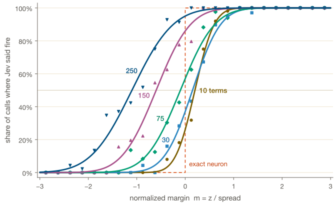
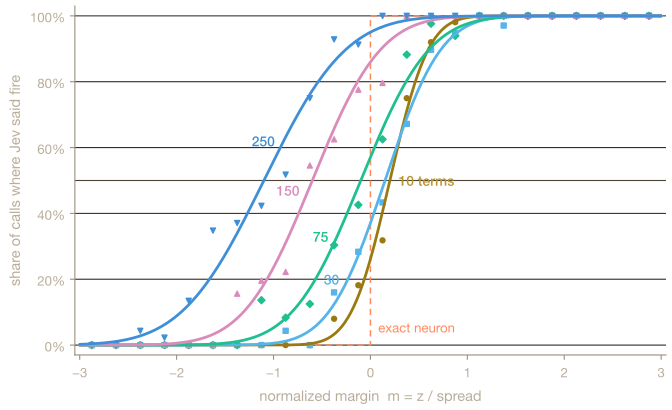
Each curve fits a shifted normal CDF, with for how sharp it is and for where it crosses 50/50:
is the standard normal CDF. This fits firing frequencies across sampled states, rather than the probability that repeated calls on one fixed state will fire. The fitted values for each term count are:
| Terms | Fires when | Fires when | Sign accuracy | ||
|---|---|---|---|---|---|
| 10 | 3.2 | +0.20 | 1.9% | 91.9% | 95.1% |
| 30 | 2.2 | +0.15 | 4.8% | 92.1% | 93.6% |
| 75 | 1.8 | -0.10 | 9.5% | 96.1% | 93.3% |
| 150 | 1.8 | -0.60 | 19.4% | 98.1% | 89.1% |
| 250 | 1.5 | -1.10 | 38.8% | 100.0% | 80.9% |
Based on these experiments, Jev behaves like a noisy threshold that gets worse in two ways as the list gets longer. The curve blurs, with falling from 3.2 to 1.5, and the threshold slides below zero, so Jev starts leaning toward “fire”. At 250 terms it fires on 39% of negative totals and on every positive one, which means long-sum errors are mostly false fires. Asking the same neuron twice flipped the answer 2-5% of the time. (To reach large margins, the sampler nudges all of a neuron’s weights the same way, so the high- neurons mostly have products of the same sign.) The trouble with longer lists matches the warning in the TypeSafe docs, and my experiments also showed a bias toward firing and a tendency to repeat the same mistakes.
I had hoped to save calls by packing eight neuron states into one request under separate keys, but that changed 11–18% of the answers compared with sending each neuron alone, so I kept one request per neuron.
#The bias trick
The first time I included a bias, I wrote it as its own field next to the products:
{"bias": b, "products": [x_1 w_1, x_2 w_2, ..., x_k w_k]}With the bias written that way and drawn independently of the terms, Jev’s answer followed the bias sign 72-97% of the time, whatever the products added up to. My guess is that a separate bias key in the state makes Jev over-index on it, so one number standing apart from a long list gets more weight than the list itself.
Appending the bias to the list as one more product fixed most of it (40 neurons per cell):
| Sign accuracy per call, by format | 10 terms | 30 | 75 | 150 |
|---|---|---|---|---|
| products + separate bias | 90% | 85% | 83% | 75% |
| products with bias folded in | 95% | 85% | 85% | 90% |
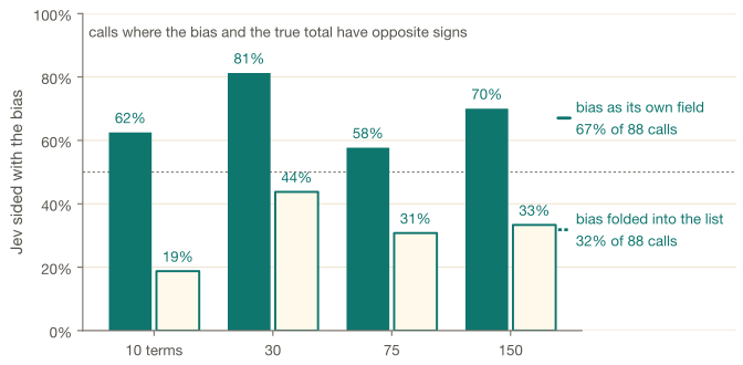
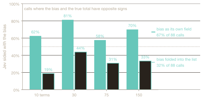
Folding the bias in looked like a formatting detail at 40 neurons per cell, but it turned out to be what let a network learn XOR at all, the function that outputs 1 when exactly one of its two inputs is 1. XOR is the smallest problem a single neuron can’t solve2, which makes it the usual first test for a network with a hidden layer, and before I could run it I needed a way to train the network.
#Backprop without a gradient
Backprop needs each neuron’s derivative, and that’s hard to formulate here, since a threshold’s slope is zero everywhere except at the jump and Jev is a remote black box anyway, so I tried two ways around it.
The first, SPSA (simultaneous perturbation stochastic approximation), skips derivatives entirely. It nudges every parameter at once by a random , measures the loss on both sides, and turns the difference into a gradient estimate. Here is every weight and bias in the network, is the training loss (defined below), and is the estimate of its gradient:
Each is an independent, equally likely random sign, one per parameter . One loss difference gives the whole estimate, and dividing by signs it per coordinate.
That’s two forward passes per step, however many parameters there are, which is the appeal. To see the catch, assume the loss changes smoothly with the weights and repeated evaluations give the same result. We can then approximate a small change using the local slope, ignoring curvature; is the true gradient the estimate is trying to recover:
The first line is the slope along the random direction, the second splits the estimate into the true component plus all the others, and the third is the noise every other parameter adds.
Under that approximation, the estimate is right on average because the random signs cancel out. The problem is that each coordinate carries the rest of the gradient as noise, so the noise grows with the parameter count while each coordinate’s signal stays put. XOR’s 2-4-1 network has 17 parameters, so every estimate is one real component mixed with 16 others. A 784-32-10 network has 25,450. Averaging perturbations cuts the variance by , so if the gradient components have comparable magnitudes, getting each coordinate’s noise down to its signal takes roughly as many perturbations as parameters. At two forward passes of 42 calls each, that example costs about 2.14 million Jev calls per training image per update. This isn’t a lower bound on SPSA’s training cost: optimization can still progress with noisy estimates, and the smooth-loss expansion doesn’t describe Jev exactly.
Call-to-call jitter adds noise to the loss difference, which SPSA divides by . Averaging repeated calls can reduce that jitter, but it won’t make the forward neuron exact: on the 3 vs 8 networks, 86–88% of misfires happened again when I repeated the input. That means Jev’s errors depend on the list in ways the margin curve misses. I didn’t test how those repeated errors affect SPSA.
The second way, the straight-through estimator3, keeps the forward pass real and fakes only the derivative. It’s the same trick used to train quantized and binarized networks, whose rounding and sign steps have no useful derivative either, and it runs the forward pass through the real neuron and in the backward pass pretends it was a smooth sigmoid of the sum it was supposed to compute. The name comes from the backward pass, which lets the gradient go straight through the neuron as if it were smooth.
The loss is binary cross-entropy on Jev’s real output, which punishes confident wrong answers hardest. Here is the right answer, 1 or 0:
For a weight from neuron into neuron , the update is a constructed surrogate gradient , built from three factors. is a neuron’s output (its ), is the logistic sigmoid, and sets how wide its slope is:
The input activation comes from the real forward pass, while the sigmoid slope stands in for Jev’s derivative. At a hidden neuron, the gradient arriving from later layers already contains their substitute derivatives too. Jev’s aggregate firing rate rises with normalized margin at a fixed list length, which made a positive slope a reasonable first try, but neither its sign nor its size guarantees a useful update for a particular list.
Here’s the backward pass in Python, from net.py, as used for the early experiments (the digit networks change the output layer’s update, described below):
# a = Jev's p; z = w·x + b, computed in codeacts, zs = forward(params, X, jev_neuron)p = np.clip(acts[-1], 1e-3, 1 - 1e-3)da = (p - Y) / (p * (1 - p)) / Y.size
for layer in reversed(range(len(params))): s = sig(zs[layer] / tau) # slope of sigmoid(z / tau), not of Jev dz = da * s * (1 - s) / tau dW, db = acts[layer].T @ dz, dz.sum(0) # flows to the earlier layer through w da = dz @ params[layer][0].Twas 1 on XOR, 0.3 on the circle and 3 on digits, where sums are larger.
For the digit network’s output neurons, I used as the training signal: Jev’s answer minus the correct label, averaged across the images and output neurons in each batch. For example, an answer of 0.2 when the label is 1 gives -0.8 before averaging. It’s another approximation in the backward pass, and it avoids the large output gradients that the BCE formula can produce when Jev is confidently wrong.
The code clips to 0.001–0.999 for the loss and residuals; on ten digits it averages ten binary losses with one-hot labels, rather than using softmax cross-entropy. Later experiments replace the hidden sigmoid slope with a slope fitted from Jev’s measured curve.
Because the forward pass stays real and only the backward pass uses the stand-in slope, this costs no extra calls. Jev’s noise reaches the gradient only through the outputs Jev actually produced, never through a loss difference divided by and spread across every parameter.
#XOR
To build up to digits, I started with XOR, which needs a hidden layer, so this network had 2 inputs, 4 hidden Jev neurons and 1 output Jev neuron. I trained three versions on the same call budget, straight-through with the bias as its own field, straight-through with the bias folded in, and SPSA, and then ran each trained network 5 more times through live Jev.
| XOR network accuracy (share of inputs right) | Seed 0 | Seed 1 | Seed 2 | Fully correct passes |
|---|---|---|---|---|
| straight-through, separate bias | 75% | 50% | 70% | 0/15 |
| straight-through, folded bias | 95% | 100% | 100% | 14/15 |
| SPSA | 75% | 65% | 80% | 3/15 |
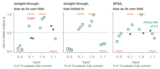
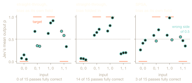
Moving the bias into the list took XOR from 0 of 15 fully correct passes to 14 of 15. SPSA ran with the bias as its own field, and against the matching straight-through row it came out slightly ahead on XOR, which is too close to call at 17 parameters. The larger network raised the scaling concern above, so I used straight-through for everything after; this XOR comparison doesn’t establish how well SPSA could train it.
What was interesting was seed 0 with the folded bias, which works on live Jev (4 of 5 passes perfect) even though its weights fail XOR when I run them through an exact step neuron. It had learned a solution for how Jev actually behaves, one that’s wrong under ideal arithmetic. One seed doesn’t prove anything, but it suggested the control I used for everything after, which is to train one network through Jev and an identical one with an exact neuron, then run both on Jev.
#Points inside a circle
Another common test is the circle, where points in a square are labeled by whether they fall inside a circle of some fixed radius. The network is 2 inputs, 6 hidden Jev neurons and 1 output Jev neuron, trained for 150 steps on 250 points and tested on 250 others, with the live scores averaged over two passes.
For each seed I trained a second network from the same starting weights with an exact step neuron, and then swapped Jev in:
| Network accuracy on 250 points, by seed | Trained through Jev, run on Jev | Trained exact, run exact | Trained exact, run on Jev |
|---|---|---|---|
| 0 | 84.2% | 93.2% | 47.2% |
| 1 | 86.2% | 90.0% | 47.2% |
| 2 | 88.4% | 81.2% | 70.2% |
For reference, a linear classifier gets 62.4% on the same points, and two of the three exact-trained networks drop below it once Jev runs them.
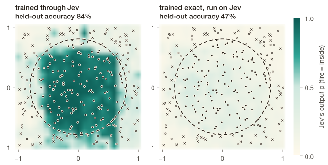
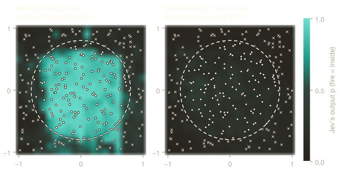
On the right, the exact-trained network never pushes Jev’s output above 0.5 anywhere, so it calls every point outside. The Jev-trained boundary on the left is blocky and lopsided, but it roughly follows the circle.
The Jev-trained weights also scored lower on an exact neuron (77-87%) than on Jev itself. That was the first real sign that the network was learning Jev’s shortcomings along with the boundary.
#Digits with the sum in code
With XOR and the circle working, I moved to the problem I cared about, MNIST4, a dataset of 28 by 28 grayscale images of handwritten digits, and the task is to say which digit, 0 through 9, each image shows. Every pixel is one input, so the network sees 784 numbers, and about 150 of them are nonzero in an average image, which is right where Jev’s adding gets bad.
The classifier I built towards is a 784-32-10 network, where the 784 pixels feed 32 hidden Jev neurons and those feed 10 output Jev neurons, one per digit, with the prediction going to the output with the highest and ties broken randomly with a fixed seed, never by the intended sum. Each hidden neuron sends Jev one product for each inked pixel, about 150 for a digit, plus its bias, and each output neuron sends the products of its weights with the 32 hidden answers.
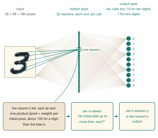
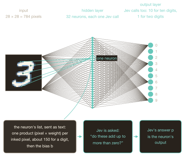
Before letting Jev add all those pixels, I tried the opposite extreme, where is computed in code and Jev only answers whether that one number is positive.
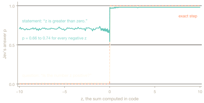
Jev is still a language model underneath, so the way you phrase a question matters, even for something this simple. I swept 2,181 values of with the question phrased as a statement (“z is greater than zero.” against “z is zero or less.”), and Jev returned 0.66-0.74 for every negative , which is a clean step with its low side above 0.5, so a thresholded neuron said yes to everything. Rewording it as a question, “Is the number z positive?”, gave 0.01-0.05 for and 0.99 for , correct on every value within ±10.
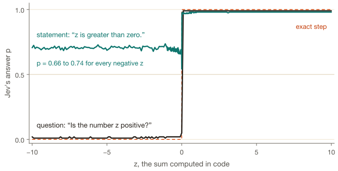
With that question, I trained a 784-32-10 network locally with an exact step neuron and then replaced every neuron with a Jev call:
| 1,000 images | Digit accuracy, exact step | Digit accuracy, Jev | Hidden sign accuracy | Output sign accuracy |
|---|---|---|---|---|
| Validation | 77.5% | 77.0% | 99.95% | 99.89% |
| Test | 78.5% | 79.1% | 99.96% | 99.92% |
With a single number to judge, Jev behaves like an exact step, so there are almost no Jev mistakes for training to compensate for, and this gives me a baseline of about 77–79% for this architecture and training recipe on 1,000 images.
#Digits with Jev doing the sum
To build up to classifying all ten digits, I started with pairs of digits and a 784-32-1 network, with the same 784 inputs and 32 hidden neurons but a single output neuron that picks between the two digits. Every neuron, hidden and output, gets the full products list, so hidden neurons add about 150 products each, and the output neuron adds 33 (32 hidden activations times their weights, plus the bias). I ran two pairs, 0 vs 1 and 3 vs 8, with one seed each, 500 training and 500 validation images and 5 epochs, with live scores averaged over two validation passes.
| Pair | Network | Pair accuracy, exact neuron | Pair accuracy, live Jev | Hidden sign accuracy | Output sign accuracy |
|---|---|---|---|---|---|
| 0 vs 1 | trained through Jev | 99.2% | 99.4% | 99.4% | 99.6% |
| 0 vs 1 | trained exact, swapped | 99.4% | 91.5% | 96.4% | 84.5% |
| 3 vs 8 | trained through Jev | 94.4% | 94.2% | 93.0% | 97.5% |
| 3 vs 8 | trained exact, swapped | 92.8% | 67.8% | 86.9% | 91.6% |
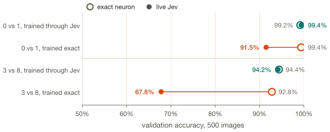
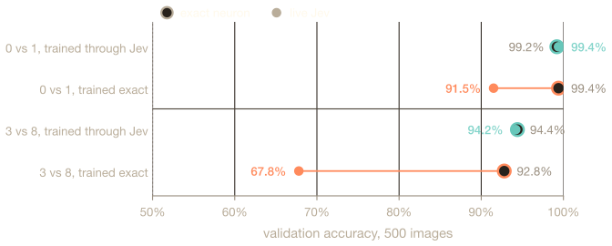
With exact neurons, the two networks score within 1.6% of each other.5 On live Jev, the network trained through Jev gets 99.4% on 0 vs 1 against its twin’s 91.5%, and 94.2% on 3 vs 8 against 67.8%. That 26.4% gap compares the two networks on Jev. I’ll use “swap gap” for a different comparison: the exact-trained network’s drop from 92.8% on exact neurons to 67.8% on Jev, or 25.0%. A local mock neuron, fitted to the error curve from the adding experiments, had predicted 93.6% and 76.5% on 3 vs 8, so it got the trained network about right and the swapped one almost 9% too high.
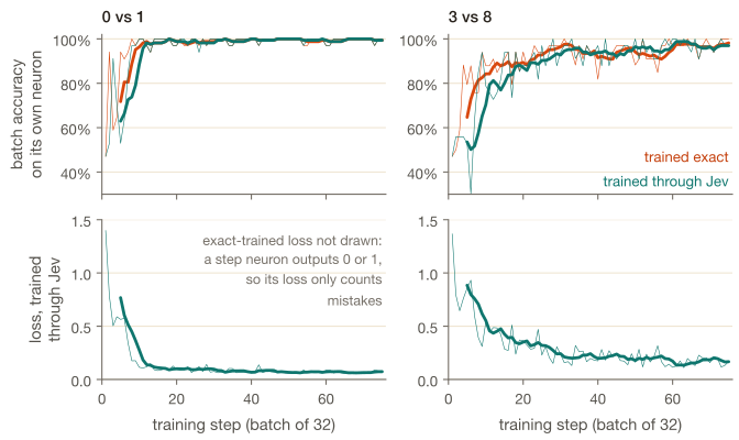
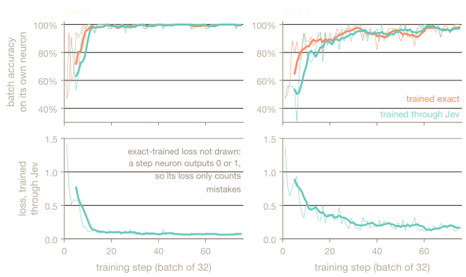
That’s one seed per pair on 500 images, so the next run had to be bigger.
#All ten digits
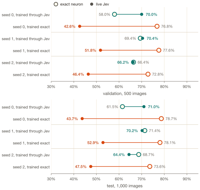
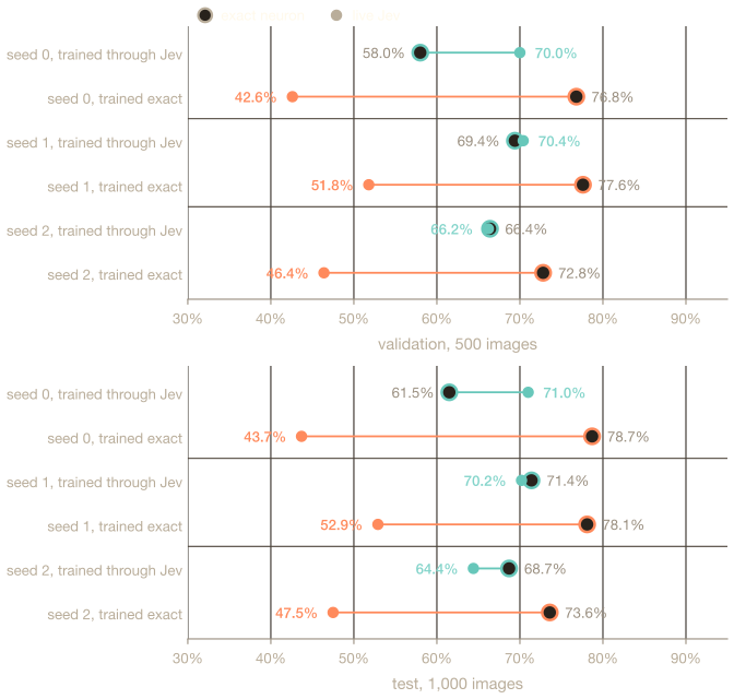
With the pairs working, I moved to all ten digits with the full 784-32-10 network, where all 42 neurons get full products lists. I trained it on 1,000 images for 10 epochs with the same settings as the two-digit runs, three seeds, each with a swapped twin trained from the same starting weights on an exact neuron. Test accuracy on 1,000 images:
| Digit accuracy, by seed | Trained through Jev, on Jev | Same weights, exact neuron | Trained exact, on Jev | Trained exact, exact neuron |
|---|---|---|---|---|
| 0 | 71.0% | 61.5% | 43.7% | 78.7% |
| 1 | 70.2% | 71.4% | 52.9% | 78.1% |
| 2 | 64.4% | 68.7% | 47.5% | 73.6% |
| Mean | 68.5% | 67.2% | 48.0% | 76.8% |
The accuracy gap is 17–27% on every seed, even though the swapped twin is the better network on paper, and in the hidden layer, neurons fired as intended 91.1% of the time in the Jev-trained networks and 84.9% in the swapped ones.
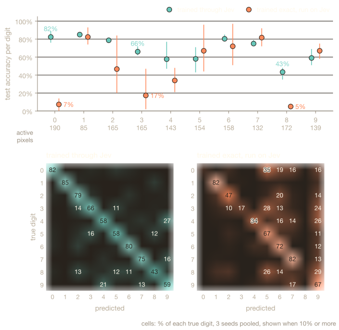
The swapped networks also don’t fail evenly, and they nearly stop predicting 0, 3 and 8 (7%, 17% and 5% correct). I think that’s because those digits have the most ink, so they produce the longest sums, where Jev’s yes-lean is strongest. The Jev-trained networks get 82%, 66% and 43% on those same digits.
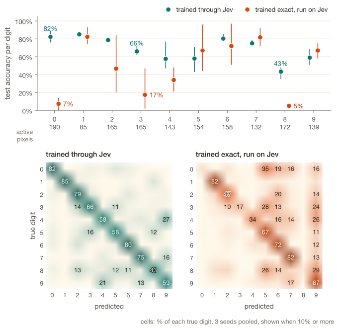
Training through Jev still has a price, since the Jev-trained networks average 68.5% against 76.8% for the matching exact-trained networks on their own neurons.
#Understanding how the weights adapt
Based on these results, I wanted to understand how the networks were learning around the places where Jev falls short. On random 150-term states, Jev gets the sign right 80-90% of the time, but inside the Jev-trained two-digit networks, where hidden neurons also add about 150 terms, it gets it right 93-99% of the time. The model, list length and wording are all the same, so the only thing training changed is which sums Jev gets asked about.
The margin curves suggested an explanation: training might move sums away from the region where Jev makes mistakes. The live forward pass makes those mistakes matter to the loss, although the surrogate updates aren’t known to follow the gradient of the true expected loss. The fitted firing curve is:
This is a population fit over lists with a given margin and length, not an independent firing probability for every fixed list.
Larger margins often put sums in regions where Jev is more reliable, though its shifted threshold makes positive and negative margins of the same size unequal. An exact neuron fires the same way at 0.01 and at 40, so training on it doesn’t directly penalize states that Jev finds difficult. That made margin growth a plausible explanation to check, rather than an objective I could claim the weights must be maximizing.
To check this, I tracked how many hidden sums sat within one spread of zero () each epoch, using the recorded training calls and a local replay of the exact-trained twins:
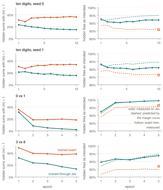
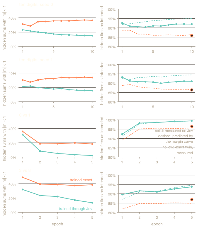
On 3 vs 8, the share of hidden sums with fell from 32% to 13% when training through Jev, and only from 49% to 38% when training exact. On 0 vs 1 it went from 31% to 2%, against 36% to 18%. The margin curve alone predicts the exact twins’ live fires-as-intended rate to within 2.4%.
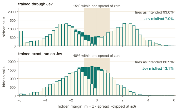
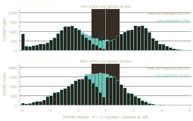
Similarly, you can see it in the weights of the two 3 vs 8 networks, which started from the same random weights:
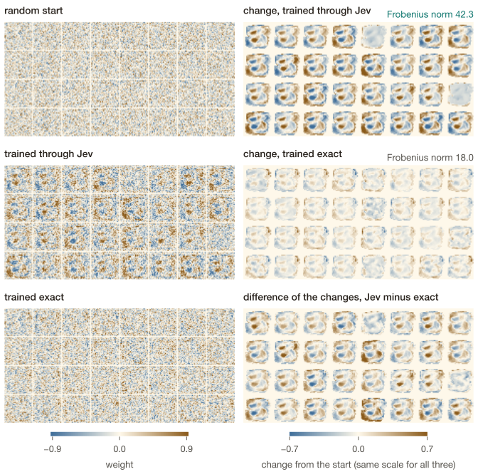
Training through Jev moved the first layer more than twice as far (a change of 42.3 against 18.0, in Frobenius norm), and the change draws clear 3 and 8 templates, marking the gaps on the left of a 3 where an 8 has ink. The exact-trained weights still look like the random start.
I expected the Jev-trained sums to drift negative, to compensate for Jev’s yes-lean, but they drift the other way, and on ten digits the median neuron’s mean sum moved +4.1 when trained through Jev and -3.5 when trained exact. My guess is that Jev’s almost never reaches 0 or 1 (across every recorded call, 0.4% are at or below 0.02 and 0.9% at or above 0.98), so even after a correct prediction, Jev can leave a much larger error signal than the exact network does (its outputs are clipped to 0.001–0.999, so its residuals don’t vanish either, but they’re far smaller). My guess is that this keeps the weights moving, like logistic regression. There might be some evidence for it, since a simulated neuron reproduces the drift only when its output is squeezed inside 0.03-0.97, and it does so with or without the threshold lean.
Training also tolerates the misfires that remain, since even at 93% on 3 vs 8, Jev is wrong on 7% of hidden evaluations and the network still gets 94.2%. The measurements show both fewer difficult sums and successful digit predictions despite remaining misfires; they don’t isolate a separate learned error-correction mechanism.
The margin curve doesn’t explain all of it, though, because on ten digits the Jev-trained hidden neurons fire as intended 90-92% of the time, where their margins say they should manage 94-95%. Perhaps the margin curve is too simple a model of Jev, or my formulation of it is missing something, but something else about Jev was reducing sign accuracy.
#A few more of Jev’s quirks
The bias was the first quirk I found, and it isn’t in Jev’s docs. By this point I had about 1.47 million Jev results, each with a known true sign, so I went looking for more.
A logistic model of Jev’s answer, fitted on the margin plus a few features of the list, picks out three things beyond the length blur and the yes-lean. Jev’s answer depends on the balance of positive and negative terms, so at 120-199 terms a list where 60% of the terms are positive gets pushed toward “fire” about as much as moving the total 0.6 spreads. It gives the first third of the list slightly more weight than the last third (5-24% more). It also doesn’t behave like a simple prefix-only adder in these tests, since when a partial sum of the first few terms has the wrong sign, Jev sides with the full total most of the time. None of these rival the margin, though. Adding them improves agreement with Jev’s answers by only 0.1–0.4%, and they describe what moves Jev’s answer without saying anything about how it computes.
To test whether these effects were real, I built trap states and matched controls, 200 of each. Each pair has the same term count and spread, and usually the same total. The mirror comparison flips the sign of every number, which reverses the total.
Here’s one actual state from the position test, with a single +4.92 among 74 small negatives:
Example Trap State
{ "products": [ -0.06, -0.10, -0.13, -0.11, -0.06, -0.11, -0.08, -0.06, -0.15, -0.09, -0.07, -0.06, -0.13, -0.08, -0.06, -0.10, -0.11, -0.10, -0.13, -0.07, -0.07, -0.11, -0.09, -0.07, -0.15, 4.92, -0.05, -0.09, -0.13, -0.07, -0.07, -0.12, -0.08, -0.10, -0.13, -0.06, -0.09, -0.10, -0.10, -0.13, -0.09, -0.10, -0.14, -0.13, -0.14, -0.09, -0.09, -0.09, -0.07, -0.12, -0.15, -0.15, -0.14, -0.07, -0.09, -0.11, -0.13, -0.14, -0.06, -0.06, -0.09, -0.12, -0.11, -0.13, -0.08, -0.15, -0.11, -0.14, -0.13, -0.11, -0.05, -0.07, -0.13, -0.11, -0.11 ]}The negatives add up to -7.47, so the total is -2.55. Jev returned and fired, getting the sign wrong. In the paired call, the +4.92 was at the end, with every other number still in the same order, and Jev returned . The total and spread were unchanged, but this time it got the sign right.
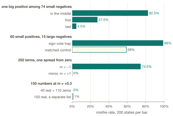
Three of the traps fooled Jev far more often than their controls. A list of mostly small positives with a few large negatives, whose total is negative, fires 99% of the time, which supports an effect of sign count without identifying how Jev computes internally. A long list one spread below zero fires about three times in four, while its mirror image above zero never fails. The strongest effect was position, where one big positive number buried in the middle of 74 small negatives fools Jev 82.5% of the time, against 27.5% when it comes first and 4.5% when it comes last. The regression had me expecting the last slot to be the most misleading, and it turned out to be the safest.
#Trying laya
Since Jev took off, several other System-1 models have appeared, and Ollaya runs open-weight ones locally behind the same API. That made each of them another backend I could run locally, and I wanted to know whether any model used this way comes with Jev’s quirks. In small experiments the base models mostly can’t add, and laya (421M parameters) and von answer “fires” to nearly every folded sum, for 47-65% sign accuracy, and decider is a partial adder at 60-80%.
laya even fails the scalar version, getting the sign right 52% of the time when asked whether is greater than zero, with a jagged, V-shaped response. Even so, when I put laya in every hidden neuron of a 3 vs 8 network, with the sum computed in code, a conventional sigmoid output neuron and backprop going through a smoothed copy of laya’s measured curve, the network gets 96.0% on live laya, while the exact-trained twin run on laya is a coin flip at 50.0%. In this setup, training could use an activation that was a poor sign test but still varied with the input. (To be fair to laya, most of that 52% was the question format. Asked as a neutral two-option choice instead of yes/no, it gets the sign right on every sampled from -10 to 10.)
#Two questions per neuron
I also tried shrinking the swap gap by making Jev less wrong, without retraining Jev at all. I tried a few fixes on 3 vs 8, each with the exact-trained network swapped onto the new neuron. Shifting the bias sent to Jev by the measured threshold drift closed about 30% of the original accuracy gap (25%).
The fix that worked borrowed laya’s neutral-choice question and asked Jev that too. Each call now carries the usual yes/no question and a two-option question (“above zero” against “below zero or equal”), and the neuron’s output is their average. Yes/no leans toward “fire” and the choice leans toward “below”, so averaging them cancels most of both. The exact-trained network keeps 88.2% on that neuron against 67.8% on plain yes/no, which drops the gap from 25.0% to 4.6%. In the network trained through it, hidden neurons fire as intended 96.0% of the time, which makes it the most faithful Jev neuron I’ve built, and accuracy is 95.2% (94.2% before). That’s one seed per arm, and the new trained arm also uses a measured-curve surrogate, so I wouldn’t infer much from the 1% training gain. Changing the question format on the fixed exact-trained network produces a much larger improvement.
Jev’s repeat behavior gives some context for why another question format helped more than repeating the same one. When Jev misfires on a call, it misfires on the same call again 86-88% of the time. If each repeat were an independent draw at the misfire rate the margin curve predicts for that call, a repeat would misfire only 52-59% of the time. Its jitters between repeats, but the decision barely moves, so the margin curve misses input-specific behavior. Repeating or rewording the question tends to reproduce the same wrong answer, while a different question format makes different errors.
#How far the weights bend
Another question I could answer offline was whether a more faithful neuron leaves the weights closer to the exact solution. I also included a fine-tuned version of laya in this comparison because it made fewer arithmetic mistakes. To measure it, I defined a network’s bend as how far its first-layer weight change sits from its exact twin’s, relative to the size of the twin’s change. is the first layer’s weight matrix:
is the change from the shared random start, and both norms are Frobenius norms. Some comparisons also change the backward rule: the averaged neuron uses a measured-curve slope while its exact twin uses a sigmoid slope, so bend reflects the training recipe as well as the forward neuron.
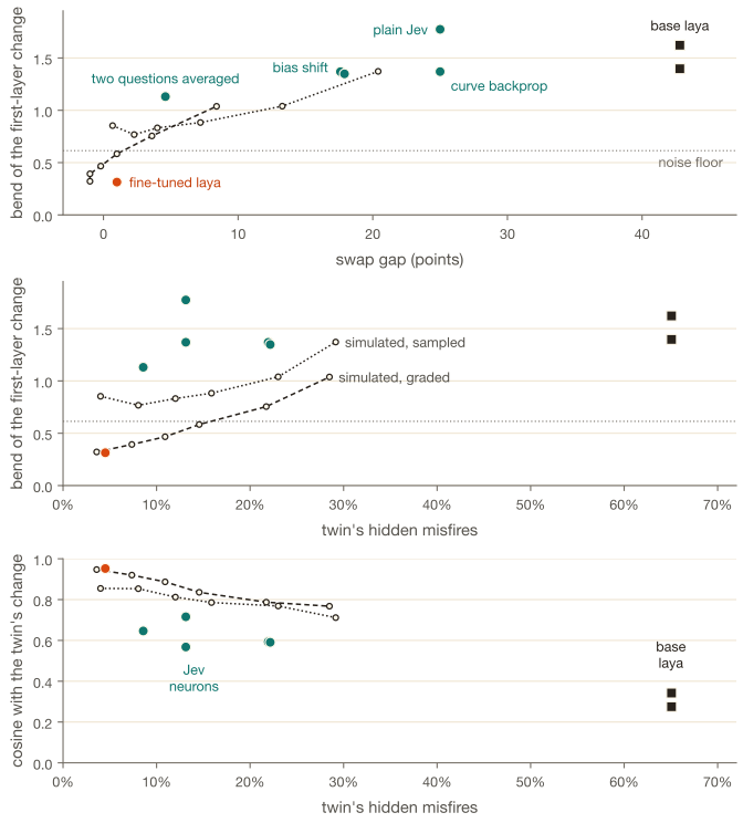
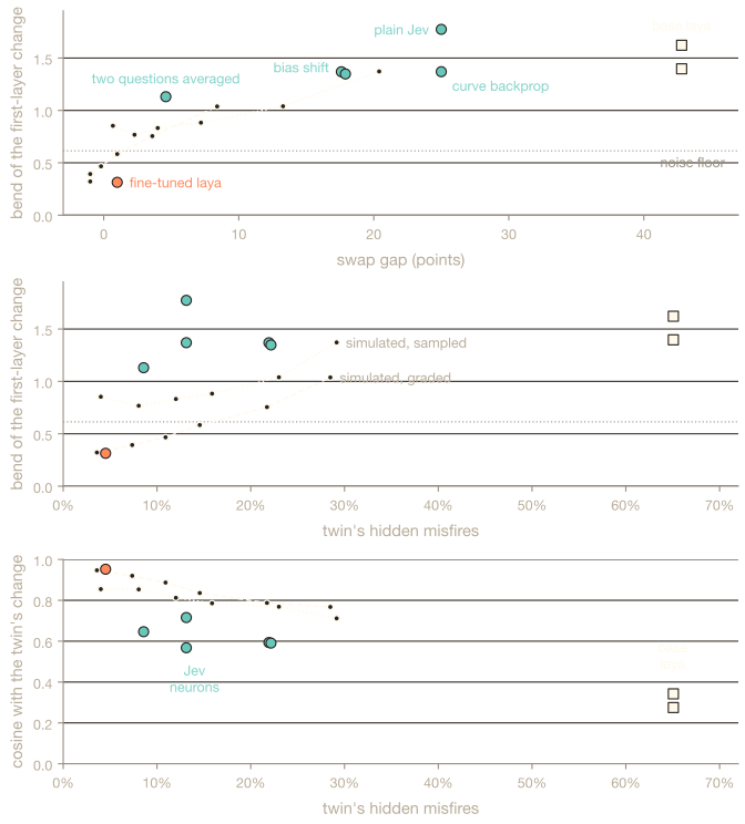
The ordering matches, with plain Jev bending 1.77, the averaged neuron 1.13 and fine-tuned laya 0.31, but it isn’t a clean relationship. The bias shift cut the swap gap from 25% to 18% without bending any less than the unshifted neuron trained the same way, and at similar misfire rates (14.6% for the graded simulator, 15.9% expected for the sampled one, against 13.1% for Jev), a simulated neuron built from Jev’s own margin curve bends 0.58 to 0.88, half of what Jev does or less. I think that means Jev has some behavior beyond its margin curve that I haven’t identified yet.
Training also doesn’t aim where I expected, since in trained networks 92-99% of Jev’s hidden misfires are false fires, yet training doesn’t target them. The Jev-trained 3 vs 8 network pushed its sums out on both sides (median around -2.5 and +2.2), and relative to its exact twin it gained more margin on the positive side than the negative, the opposite of compensating for a yes-lean.
To see where the Jev-specific change is concentrated in the weights, I took, for each pixel, the size of the difference between the Jev-trained and exact-trained first-layer changes across all 32 hidden neurons:
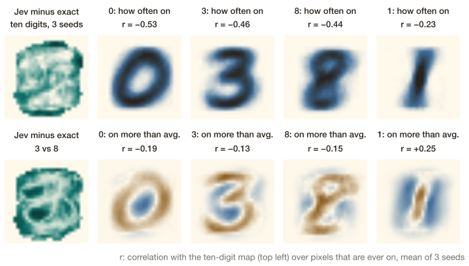
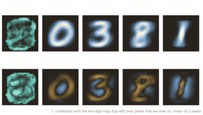
On ten digits it’s a ring at the edge of the digit area, and it’s nearly the same map in all three seeds (r 0.96-0.97 between seeds that started from different random weights). It runs opposite to how often a pixel is on (r -0.50 to -0.54 over pixels that are ever on), and weights on pixels that are on in 1-10% of images moved 1.4-1.5 per weight (rms) in the Jev-trained networks, against 0.8-0.9 on pixels that are on in more than 40%. The exact twins have the same profile at about a quarter of the size.
I think Adam6 may help explain why rarely-on pixels move so much, though I haven’t isolated its effect. It scales updates using each weight’s gradient history, so even a small, steady gradient can produce a substantial step. Jev’s graded outputs keep residuals alive after a prediction is correct, but the exact networks retain small residuals too because the implementation clips probabilities to 0.001–0.999. Rare gradients also aren’t necessarily steady, so I’d need an optimizer comparison to test this explanation.
That weakens one explanation for the 0, 3 and 8 collapse. If Jev training had rewritten the weights those digits depend on, the difference would sit on their pixels, and the map doesn’t show that pattern. Weight movement alone doesn’t tell me a pixel’s causal effect on a prediction. The pixels 0, 3 and 8 use more than average are slightly avoided (r -0.11 to -0.20), and their on-pixels carry about half as much of the difference as their share of the pixels. Long lists remain one possible explanation, with 190, 165 and 172 active pixels on average against 85 for a 1.
#Training on 5,000 images
I then put the two-question neuron on the full 784-32-10 network and gave it 5,000 training images instead of 1,000, with one seed and eight epochs, tested on 2,000 images. The split also changed, and the Jev arm used a measured-curve surrogate while the exact twin kept the sigmoid surrogate.
| Digit accuracy, 2,000 test images | On Jev | Same weights, exact neuron |
|---|---|---|
| Trained through Jev | 84.6% | 70.0% |
| Trained exact, swapped | 52.6% | 83.9% |
That’s 84.6% on Jev, up from 68.5%, and above the 77-79% an exact neuron reached at 1,000 images. The Jev-trained weights now do worse on a perfect neuron than on Jev, which means they’ve specialized to the neuron they had.
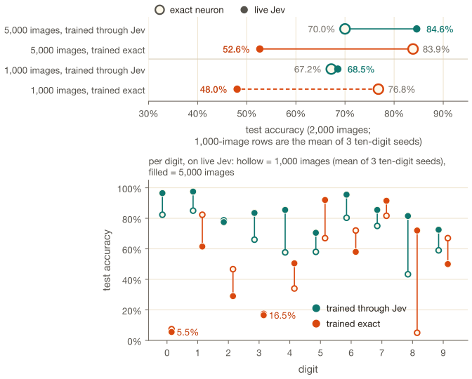
I expected the swap gap to shrink here, since the two-question neuron had cut it from 25% to 4.6% on 3 vs 8. Instead it grew, from 28.8% at 1,000 images to 31.2%. The swapped network’s hidden neurons agree with the intended sign 93.5% of the time, against 90.8% in the Jev-trained network, so hidden sign agreement alone doesn’t explain the failure. In the swapped network, none of the ten output neurons fires on 97.8% of images, so every prediction comes down to which “no” is the least confident, making the ordering of those probabilities matter even when all ten signs agree. The Jev-trained network gets an output neuron to fire on about 40% of images. The long-list digits also still fail in the swapped network (6% of 0s and 17% of 3s), so Jev is still wrong on the inputs this network sends it, and the output ranking is another place the swap fails. Separately swapping hidden and output layers would help isolate where those failures start.
#Sparse hidden neurons
The swapped networks kept failing on the same digits, with 0 and 3 collapsing at 1,000 images and again at 5,000 and 8 collapsing at 1,000, and they’re the digits with the most ink, so they have the longest lists. In a dense network, training can’t fix that one neuron at a time, because every hidden neuron sees every nonzero pixel, so the image sets the length of its sum and a 0 hands all 32 hidden neurons about 190 numbers whatever their weights are. Looking back at the dense networks, nothing in the Jev-trained weights was tuned to image length either, since their false fires rise with length as steeply as their exact twins’.
Another approach I decided to take was to stop sending Jev long lists, by giving each hidden neuron only a subset of the pixels. The network is 784-64-10, and each hidden neuron connects to 96 pixels, drawn at random from the 379 that are on in at least 5% of training images, with its other weights held at zero. Only connected pixels that are on in the image get sent, so a hidden call carries about 37 numbers (10th to 90th percentile 23-50), a length where Jev’s curve is sharp. The 10 output neurons stay dense, each adding all 64 hidden answers. I picked random fields over local patches after a local comparison, where the two were within 1–2% on accuracy but a random field gives every neuron a similar share of the ink, while a patch at the edge of the digit sends almost nothing and one at the center sends 60 or more. I doubled the hidden layer to 64 to make up for each neuron’s narrower view, and kept the two-question neuron.
I trained it on 1,000 images for 6 epochs, one seed, with an exact-trained twin from the same start, and tested both on 1,000 images:
| Digit accuracy, 1,000 test images | On Jev | Same weights, exact neuron |
|---|---|---|
| Trained through Jev | 85.3% | 75.7% |
| Trained exact, swapped | 65.8% | 72.6% |
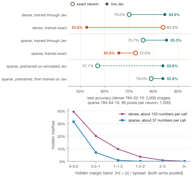
85.3% is the highest observed score so far, with a fifth of the dense run’s training data, though one seed and different test samples don’t establish an improvement over 84.6%. In hindsight that fits the TypeSafe docs, which say the less adding Jev has to do, the more reliable it is. With shorter lists going to Jev, the swap gap fell from 31.2% to 6.8%. The swapped network no longer loses 0 (99%, its best digit), and loses 8 and 6 instead (29% and 38%).
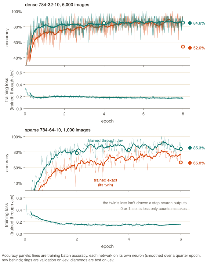
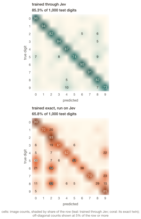
I expected sparsity to help by making the hidden neurons more accurate, and that isn’t quite what happened. Shorter sums are sharper, so at the same margin a 37-number call misfires far less often than a 153-number one (pooling both arms, 7.0% against 20.1% between 0.5 and 1 spreads from zero, and 0.7% against 9.7% between 1 and 1.5). But the sparse networks’ sums also sit closer to zero, at about half the dense network’s median margin, so their hidden neurons fire as intended about as often as before (90.7-91.6%). Nearly all the remaining misfires are within one spread of zero, although their downstream effect still depends on the outgoing weight times the change in activation. The output layer also behaves better, and where the dense swapped twin had no output firing on 97.8% of test images, the sparse one has none on 81.0%, though the sparse output neurons also add 64 hidden answers instead of 32, and I didn’t test whether the sparse fields or the wider layer made the difference.
Because several things changed at once, I don’t know which one produced the result. Connectivity, width, question format, backward rule, output initialization scale and training schedule all differ from the 1,000-image dense run (68.5%), and I didn’t run a dense 784-64-10 network to separate them. It’s also a single seed, while the three ten-digit seeds spread 6.6% on Jev, and the dense network used a different test sample, so comparing 85.3% with 84.6% crosses samples.
#Training on Jev’s curve
Running these experiments left me with a lot of recorded Jev answers7, including 192,000 from the two-question neuron in the 5,000-image run. I fitted a simulated neuron to them: Jev’s margin curve, blurred and shifted per layer, with its output squeezed into 0.04-0.96 the way Jev’s is. It’s deterministic, so it repeats its answers, although that doesn’t mean it reproduces Jev’s specific repeated mistakes. Then I trained the sparse network entirely through the simulator.
On real Jev, the simulator-trained network gets 83.8% on the same 1,000 test images, while the exact-trained twin keeps 65.8%, so the simulator gives an 18% accuracy gain, compared with 19.5% from training directly through Jev. Two epochs of fine-tuning on real Jev raised validation from 81.0% to 83.4% and left test at 83.8%. With the same amount of training on Jev, the pretrained network leads training from scratch on Jev by 5% on validation (83.4% against 78.4%). On one seed, neither the fine-tuning gain nor the 1.5% separating 83.8% from 85.3% is established.
There’s also a test-set limitation: I fitted the simulator on responses from the earlier dense run’s test images, and 187 of them overlap this 1,000-image evaluation. Their digit labels weren’t used for the fit, but responses derived from the inputs were, and the simulator also informed sparse architecture selection. A fresh, disjoint evaluation is needed before treating these scores as fully held out.
The simulator isn’t a model of Jev in general, though, because while it predicts Jev well for weights trained through it, 84.8% on the simulator against 83.8% on Jev, for the exact-trained network it predicts 35.6% on validation where Jev gives 66.4%. My guess is that a curve fitted on margin alone can’t capture how Jev errs, since Jev’s answers jitter between calls and its mistakes depend on the specific list. A network trained through the simulator ends up with sums where the two mostly agree, and one that never saw a graded neuron doesn’t. I’d use it to pretrain networks, but I wouldn’t trust what it predicts about Jev for a network it didn’t train.
#Caveats
The whole project cost about $230 in Jev calls, and most of its running time went to waiting on those calls because of rate limits. The 1,000-image ten-digit result is the only MNIST comparison with three seeds and a test set behind it. The two-digit results are single runs on 500 validation images, and the larger and sparse runs changed several parts of the training recipe at once. The circle networks weren’t converged, so the circle’s swap gap points the same way on every seed but its size is noisy.
I also don’t know how correlated Jev’s errors are across neurons in the same image, which my mock and simulated neurons both assume away. The 84% in the opening is also Mustafa’s reported figure for his ALU, which I didn’t measure myself.
#Try it yourself
I built a demo so you can draw your own digit and watch it run through the sparse network on real Jev calls! The page shows each neuron’s intended sum next to Jev’s answer, so you can see exactly where Jev gets the arithmetic wrong and the network gets the digit right anyway.
#Footnotes
-
The API reference documents answers and token usage, with no gradient or logit output. Noul is TypeSafe’s name for the probability-valued answer. ↩
-
Minsky and Papert’s Perceptrons (MIT Press, 1969) proved that a single-layer perceptron can’t compute XOR, which is part of why hidden layers became the standard answer. ↩
-
Bengio, Léonard and Courville 2013 describe straight-through estimators for stochastic and hard-threshold neurons. Courbariaux et al. 2016 use one to train binarized networks, whose weights and activations are all +1 or -1. ↩
-
LeCun, Bottou, Bengio and Haffner 1998 introduced MNIST, and the dataset page has the files. I used the standard 60,000-image training set and 10,000-image test set, drawing smaller samples from them. ↩
-
Accuracy differences written as % are absolute differences between scores (percentage points), not relative percentage changes. ↩
-
Kingma and Ba 2014. Adam uses bias-corrected first and second moments of each parameter’s gradient; a small but steady gradient can therefore still produce a substantial update. ↩
-
The code, trained weights, results and figure scripts are at github.com/iamrajjoshi/jevrons. The raw response journals aren’t published, so readers can’t replay every call-level analysis from the public repo. ↩